Resampling

"Resampling is the process of converting a signal from one sampling rate to another, while changing the information carried by the signal as little as possible. When applied to an image, this process is sometimes called image scaling." (source).

The idea behind resampling is to reconstruct the continuous signal from the original sampled signal and resample it again using more samples (which is called interpolation or upsampling) or fewer samples (which is called decimation or downsampling). In the context of image processing the original sampled signal is the source image (where the luma and chroma-values of the pixels are the samples). Interpolation is called upsampling and decimation is called downsampling (or subsampling).

Resampling

The Nyquist–Shannon sampling theorem

The Nyquist–Shannon sampling theorem asserts that the uniformly spaced discrete samples are a complete representation of the signal if its bandwidth is less than half its sampling rate. (source: wikipedia). In theory the continuous signal can be reconstructed as follows (n runs over the integers)

s(x) = sum_n s(n*T) * sinc((x-n*T)/T), with sinc(x) = sin(pi*x)/(pi*x) for x!=0, and = 1 for x=0

with fs = 1/T the sampling rate, s(n*T) the samples of s(x) and sinc(x) the resampling kernel. Although in practice, signals are never perfectly bandlimited, nor can we construct a perfect reconstruction filter (because an image always has a limited number of pixels), we can get as close as we want in a prescribed manner. This is the reason why many resamplers are based on this construction. Note that the reconstruction filter has the following properties:

1. The reconstruction is exact for x=m*T (m integer), meaning that s(m*T) are indeed samples of the continuous signal s(x). (This follows from the fact that sinc(0)=1.)
2. The sum of the coefficients is one, thus sum_n sinc((x-n*T)/T) = 1 (this seems to be true for all x and T, but I can't find a reference for it). This implies that if all samples have the same value (say s(n*T)=y for all n), then it follows that the continuous signal itself is constant and is equal to that value. That is, s(x)=y for all x.
3. The resampling kernel, sinc(x), is maximal and equal to one for x=0. It has such a shape that the sample s(n*T) for which its location (n*T) is the closest to the value x will contribute the most to s(x).
4. The resampling kernel, sinc(x), is symmetric. That is, sinc(x) = sinc(-x). This means that the samples s(n*T) and s(-n*T) will contribute equally to s(0).
5. The resampling kernel, sinc(x), is analytic (infinitely differentiable) everywhere (source: wikipedia).

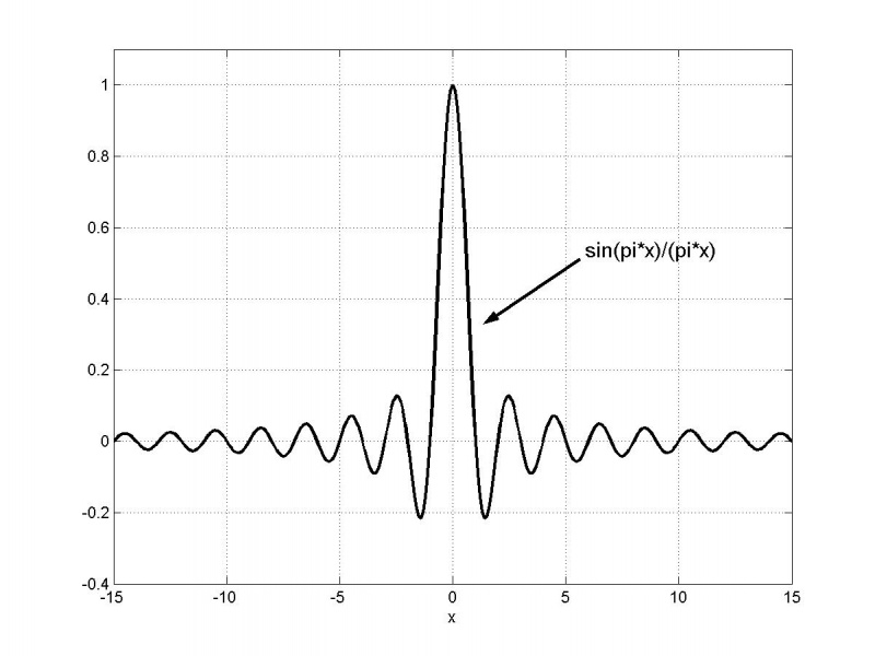
The normalized sinc kernel

As an approximation of this reconstruction function, many interpolation functions s(x) are written in the form

s(x) = sum_n s(n*T) * f((n*T-x)/T) := sum_n s_T(n) * f(n - x/T)

with f(x) the (symmetric) resampling filter (or resampling kernel) obeying some of the properties listed above and {s_T(n)}_n the samples. Unfortunately such an approximation causes artifacts such as blurring, aliasing and ringing. The possible artefacts are explained here.

Example: the bilinear resampling filter - upsampling

Let's consider a bilinear resampling filter

f(x) = 1 - |x| for |x|<1
     = 0 elsewhere

Note that this filter satisfies the properties 2, 3 and 4 that are mentioned above.

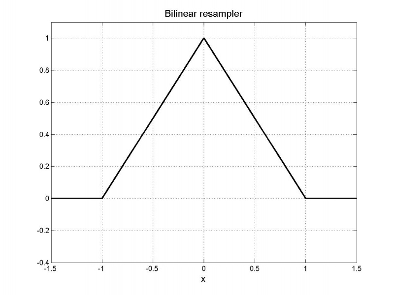
The bilinear resampling filter

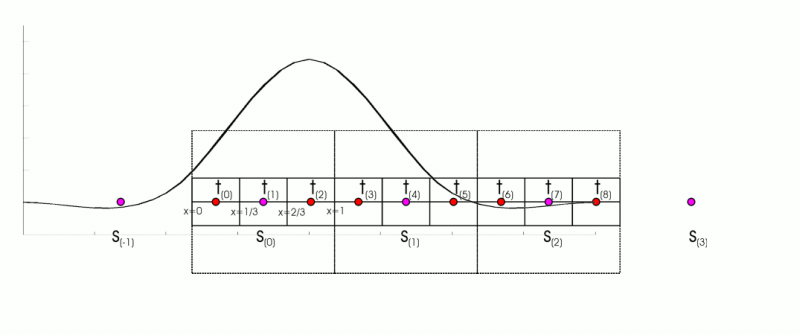
Let's upsample an image (consisting of three pixels) by a factor T=3. Thus the target image has nine pixels.

Let s_3(j) be the luma-channel (or one of the color-channels) of the j+1-th source pixel, and t(j) the luma-channel (or one of the color-channels) of the j+1-th target pixel. Two fake pixels are added: s_3(-1) and s_3(3). They will be set equal to the value of the boundary pixels: s_3(0) and s_3(2). The center pixels of the source image and the destination image (here s_3(1) and t(4)) should coincide.

When upsampling, it is assumed that a source pixel occupies an unit-square and it is centered its center. So the source pixel s_3(0) is located at [0,1[ and it is centered at x=1/2.

More generally: the source pixels are s_T(0) ... s_T(m-1) and the target pixels are t(0) ... t(n-1). The centers of the source and destination image should coincide. This means that t(c_n) = s_T(c_m) = s(c_m*T) with c_m = (m-1)/2 and c_n = (n-1)/2. This implies that

t(x) = s(x - (c_n - c_m*T)) = s_T((x - c_n)/T - c_m)

with

s(x) = sum_n s_T(n) * f(n - x/T)

In our example: T=3, m=3, n=9, thus c_m = 1, c_n = 4 and thus

t(x) = s(x - 1)

with

s(x) = sum_n s_3(n) * f(n - x/3)

For the third target pixel, for example, we will get

t(2) = s(1) = sum_n s_3(n) * f(n - 1/3)
     = s_3(-1) * f(-1-1/3) + s_3(0) * f(0-1/3) + s_3(1) * f(1-1/3) + s_3(2) * f(2-1/3) + s_3(3) * f(3-1/3)
     = s_3(-1) * f(-4/3) + s_3(0) * f(-1/3) + s_3(1) * f(2/3) + s_3(2) * f(5/3) + s_3(3) * f(8/3)
     = s_3(0) * f(-1/3) + s_3(1) * f(2/3)
     = s_3(0) * 2/3 + s_3(1) * 1/3

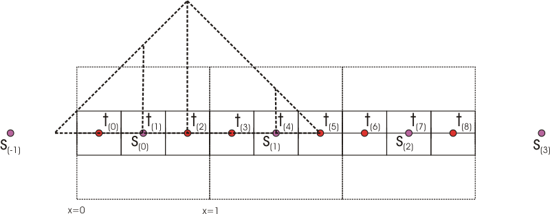
s_3(0) contributes 2/3 to the target pixel t(2), and s_3(1) contributes 1/3 to the target pixel t(2)

The remaining target pixels are given by:

t(0) = 1/3 * s_3(-1) + 2/3 * s_3(0) = f(-2/3) * s_3(-1) + f(1/3) * s_3(0) = s_3(0)
t(1) = 3/3 * s_3(0) + 0/3 * s_3(1) = f(0) * s_3(0) + f(1) * s_3(1) = s_3(0)
t(2) = 2/3 * s_3(0) + 1/3 * s_3(1) = f(-1/3) * s_3(0) + f(2/3) * s_3(1)
t(3) = 1/3 * s_3(0) + 2/3 * s_3(1) = f(-2/3) * s_3(0) + f(1/3) * s_3(1)
t(4) = 1 * s_3(1) + 0 * s_3(2) = f(0) * s_3(1) + f(1) * s_3(2)
t(5) = f(-1/3) * s_3(1) + f(2/3) * s_3(2)
t(6) = f(-2/3) * s_3(1) + f(1/3) * s_3(2)
t(7) = 3/3 * s_3(2) + 0/3 * s_3(3) = f(0) * s_3(2) + f(1) * s_3(3) = s_3(2)
t(8) = 2/3 * s_3(2) + 1/3 * s_3(3) = f(-1/3) * s_3(2) + f(2/3) * s_3(3) = s_3(2)

Example: the bilinear resampling filter - downsampling

Let's upsample an image (consisting of nine pixels) by a factor T=1/3 (thus downsample by a factor of 3), with the target image having three pixels.

We have

t(x) = s(x - (c_n - c_m*T))

with

s(x) = sum_n s_T(n) * f_T(n - x/T) 

and

f_T(n - x/T) = T * f(T*n - x)

Note that f is zero outside [-1,1] for the bilinear resampling filter, and thus it follows that for all j (and all T<1):

sum_n f_T(n - j) = T * sum_n f(T*n - j)
                 = T * (f(T-1) + f(2*T-1) + ... + f(1/T*T-1) + ... + f(1-2*T) + f(1-T))
                 = T * (T + 2*T + ... + 1 + ... + 2*T + T)
                 = T^2 * (1 + 2 + ... + 1/T + ... + 2 + 1)
                 = 2*T^2 * (1 + 2 + ... + (1/T-1)) + 1/T * T^2
                 = 2*T^2 * 1/2 * (1/T-1) * 1/T + T
                 = 1

In our example: T=1/3, m=9, n=3, thus c_m = 4, c_n = 1 and thus

t(x) = s(x + 1/3)

with

s(x) = sum_n s_1/3(n) * f_T(n - 3*x) = 1/3 * sum_n s_1/3(n) * f(n/3 - x)

For the first three pixels we obtain:

t(0) = s(1/3) = sum_n s_1/3(n) * f_T(n - 1)
     = s_1/3(-1) * f_T(-1-1) + s_1/3(0) * f_T(0-1) + s_1/3(1) * f_T(1-1) + s_1/3(2) * f_T(2-1) + s_1/3(3) * f_T(3-1)
     = s_1/3(-1) * f_T(-2) + s_1/3(0) * f_T(-1) + s_1/3(1) * f_T(0) + s_1/3(2) * f_T(1) + s_1/3(3) * f_T(2)
     = s_1/3(-1) * f(-2/3)/3 + s_1/3(0) * f(-1/3)/3 + s_1/3(1) * f(0)/3 + s_1/3(2) * f(1/3)/3 + s_1/3(3) * f(2/3)/3
     = s_1/3(-1) * 1/9 + s_1/3(0) * 2/9 + s_1/3(1) * 3/9 + s_1/3(2) * 2/9 + s_1/3(3) * 1/9

t(1) = s(4/3) = sum_n s_1/3(n) * f_T(n - 4)
     = s_1/3(2) * f_T(2-4) + s_1/3(3) * f_T(3-4) + s_1/3(4) * f_T(4-4) + s_1/3(5) * f_T(5-4) + s_1/3(6) * f_T(6-4)
     = s_1/3(2) * f_T(-2) + s_1/3(3) * f_T(-1) + s_1/3(4) * f_T(0) + s_1/3(5) * f_T(1) + s_1/3(6) * f_T(2)
     = s_1/3(2) * f(-2/3)/3 + s_1/3(3)/3 * f(-1/3)/3 + s_1/3(4) * f(0)/3 + s_1/3(5) * f(1/3)/3 + s_1/3(6) * f(2/3)/3
     = s_1/3(2) * 1/9 + s_1/3(3) * 2/9 + s_1/3(4) * 3/9 + s_1/3(5) * 2/9 + s_1/3(6) * 1/9

t(2) = s(7/3) = sum_n s_1/3(n) * f_T(n - 7)
     = s_1/3(5) * f_T(5-7) + s_1/3(6) * f_T(6-7) + s_1/3(7) * f_T(7-7) + s_1/3(8) * f_T(8-7) + s_1/3(9) * f_T(9-7)
     = s_1/3(5) * f_T(-2) + s_1/3(6) * f_T(-1) + s_1/3(7) * f_T(0) + s_1/3(8) * f_T(1) + s_1/3(9) * f_T(2)
     = s_1/3(5) * f(-2/3)/3 + s_1/3(6) * f(-1/3)/3 + s_1/3(7) * f(0)/3 + s_1/3(8) * f(1/3)/3 + s_1/3(9) * f(2/3)/3
     = s_1/3(5) * 1/9 + s_1/3(6) * 2/9 + s_1/3(7) * 3/9 + s_1/3(8) * 2/9 + s_1/3(9) * 1/9

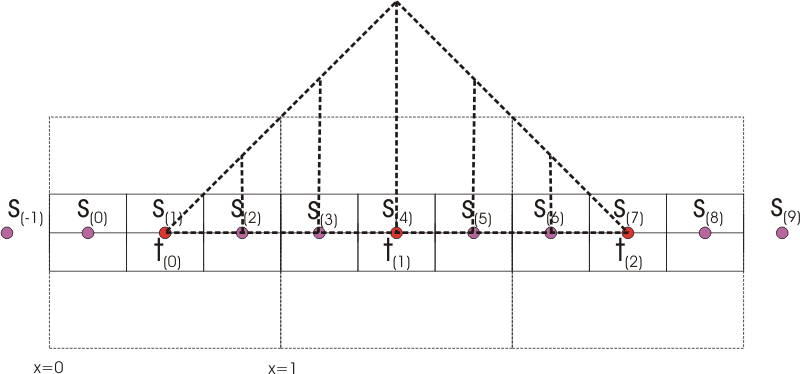
t(1) = s_1/3(2) * 1/9 + s_1/3(3) * 2/9 + s_1/3(4) * 3/9 + s_1/3(5) * 2/9 + s_1/3(6) * 1/9

Example: the bicubic resampling filter - upsampling

Suppose we want to obtain the value of t(2) in our first example. We will define our coordinate system (x,y) in such a way that s(0) is centered at x=1/2 (and thus located at [0,1[). It follows that the source pixels s(j) are centered at x=(2*j+1)/2, and the target pixels t(j) are centered at x=(2*j+1)/6. The distances from t(2) to the source pixels s(j) are (with d(x;y) = x-y):

d(s(-1);t(2)) = -4/3
d(s(0);t(2)) = -1/3
d(s(1);t(2)) = 2/3
d(s(2);t(2)) = 5/3
d(s(3);t(2)) = 8/3

Since the bicubic filter has support=2, this means that the pixels s(3) and higher don't contribute to the value of t(2). We will get

t(2) = f(-4/3) * s(-1) + f(-1/3) * s(0) + f(2/3) * s(1) + f(5/3) * s(2)
t(2) = -0.0329 * s(-1) + 0.7099 * s(0) + 0.3457 * s(1) + -0.0226 * s(2)  // b=1/3, c=1/3

t(2) = -0.0329 * s(-1) + 0.7099 * s(0) + 0.3457 * s(1) + -0.0226 * s(2) // b=1/3, c=1/3

For the other pixels we will get:

t(0) = f(-5/3) * s(-2) + f(-2/3) * s(-1) + f(1/3) * s(0) + f(4/3) * s(1)
t(1) = f(-1) * s(-1) + f(0) * s(0) + f(1) * s(1) + f(2) * s(2)
t(2) = f(-4/3) * s(-1) + f(-1/3) * s(0) + f(2/3) * s(1) + f(5/3) * s(2)
t(3) = f(-5/3) * s(-1) + f(-2/3) * s(0) + f(1/3) * s(1) + f(4/3) * s(2)
t(4) = f(-1) * s(0) + f(0) * s(1) + f(1) * s(2) + f(2) * s(3)
t(5) = f(-4/3) * s(0) + f(-1/3) * s(1) + f(2/3) * s(2) + f(5/3) * s(3)
t(6) = f(-5/3) * s(0) + f(-2/3) * s(1) + f(1/3) * s(2) + f(4/3) * s(3)
t(7) = f(-1) * s(1) + f(0) * s(2) + f(1) * s(3) + f(2) * s(4)
t(8) = f(-4/3) * s(1) + f(-1/3) * s(2) + f(2/3) * s(3) + f(5/3) * s(4)

An implementation of the resampling filters

To get implement resampling we need to know the first source pixel (also called the offset) and also the last source pixel that contributes to a certain target pixel.

Let T = n/m (m = number of source pixels, n = number of target pixels) and filter_step = min(T; 1). Thus filter_step = 1 when upsampling and filter_step = T (<1) when downsampling.

In source space, a source pixel occupies a square of length filter_step, and it is centered its center of this square. The source pixels are located at s(v) = (2*v+1)/2 * filter_step. The target pixels are located at t(v) = (2*v+1)/(2*T) * filter_step. The location, r(j), of the source pixel s_T(j) that is located directly to the left of the target pixel is given by

t(j) = s_T((j - c_n)/T + c_m)) => r(j) = floor((j - c_n)/T + c_m)  (thus rounding down to the nearest integer)

and rewriting this expression gives

r(j) = floor((j - c_n)/T + c_m)
     = floor((j - (n-1)/2)/T + (m-1)/2)
     = floor(j/T - n/(2*T) + 1/(2*T) + (m-1)/2)
     = floor(j/T - m/2 + 1/(2*T) + (m-1)/2)
     = floor(j/T + 1/(2*T) - 1/2)
     = floor(j/T + 1/(2*T) + 1/2) - 1

The offset depends on the support of the resampling filter, since the support will determine how many source pixels will contribute to the target pixel t(j). In source_space, all source pixels located in the interval [-support/filter_step, support/filter_step] contribute to the target pixel. This means that (support / filter_step - 1) pixels located to the left of the position r(j) contribute to the target pixel t(j). Thus the offset is given by

off(j) = floor(j/T + 1/(2*T) + 1/2) - 1 - (support / filter_step - 1)
       = floor(1/(2*T) - 1/2 + j/T) - support / filter_step + 1
       = r(j) - support / filter_step + 1

So, in general, the target pixel t(j) is calculated as follows

t(j) = f(b_T(j)) * s(off(j)) + f(b_T(j)+filter_step) * s(off(j)+1) + f(b_T(j)+2*filter_step) * s(off(j)+2) + ...

The value b_T(j) can be determined as follows. Note that

d(0;s(v)) = |2*v+1|/2 * filter_step
d(0;t(0)) = 1/(2*T) * filter_step
d(0;t(v)) = (2*v+1)/(2*T) * filter_step  // v>=0

The left most source pixel which contributes to t(0) is s(off(0)). It follows that

d(s(off(0));t(0)) = d(0;t(0)) + d(0;s(off(0))  // s(off(0)) is located to the left of x=0; thus off(0)<=-1
                  = 1/(2*T) * filter_step - (2*off(0) + 1)/2 * filter_step
                  = (1/(2*T) - (2*off(0) + 1)/2) * filter_step
                  = (1/(2*T) - off(0) - 1/2) * filter_step
                  = (- off(0) + 1/(2*T) - 1/2) * filter_step

Thus

b_T(0) = - d(s(off(0));t(0))
       = (off(0) - (1/(2*T) - 1/2)) * filter_step
       = (floor(1/(2*T) - 1/2) - support / filter_step + 1 - (1/(2*T) - 1/2)) * filter_step

and for j>0 (in that case off(j)>=0)

b_T(j) = - d(s(off(j));t(j)) = - (d(0;t(j)) - d(0;s(off(j))) = d(0;s(off(j)) - d(0;t(j))
       = (2*off(j)+1)/2 * filter_step - (2*j+1)/(2*T) * filter_step
       = ((2*off(j)+1)/2 - (2*j+1)/(2*T)) * filter_step
       = (off(j) + 1/2 - j/T - 1/(2*T)) * filter_step
       = (off(j) - (1/(2*T) - 1/2 + j/T)) * filter_step
       = ((floor(1/(2*T) - 1/2 + j/T) - support / filter_step + 1) - (1/(2*T) - 1/2 + j/T)) * filter_step

Note that

b_T(j) = b_T(j-1) - 1/T * filter_step

(if the right-hand side is smaller than or equal to "-support/filter_step" then one (or 1/filter_step) should be added to the right-hand side).

AviSynth's implementation

The pseudocode in AviSynth is as follows

// resample_functions.cpp
// the function GetResamplingPatternRGB is called twice:
// if source_height/target_height < source_width/target_width then the clip is resampled vertically first, then horizontally (and the other way around).
int* GetResamplingPatternRGB( int original_width, double subrange_start, double subrange_width,
int target_width, ResamplingFunction* func, IScriptEnvironment* env )

/**
* This function returns a resampling "program" which is interpreted by the 
* FilteredResize filters. It handles edge conditions so FilteredResize 
* doesn't have to. 
**/

the function returns a pointer to cur, where
// *cur = [fir_filter_size,
//  start_pos(j=0), f(b_T(j=0)[0])/total(j=0), f(b_T(j=0)[1])/total(j=0), ..., f(b_T(j=0)[fir_filter_size])/total(j=0),
//  start_pos(j=1), f(b_T(j=1)[0])/total(j=1), f(b_T(j=1)[1])/total(j=1), ..., f(b_T(j=1)[fir_filter_size])/total(j=1),
//  ...
//  start_pos(j=n-1), f(b_T(j=n-1)[0])/total(j=n-1), f(b_T(j=n-1)[1])/total(j=n-1), ..., f(b_T(j=n-1)[fir_filter_size])/total(j=n-1)]
filter_step = min(T; 1)  // T = n/m
filter_support = support / filter_step
fir_filter_size = ceil(2*filter_support)
int* result = (int*) _aligned_malloc((1 + target_width*(1+fir_filter_size)) * 4, 64);
int* cur = result;
*cur++ = fir_filter_size;

pos_step = 1/T
//  pos(j) = 1/(2*T) - 1/2 + j * pos_step
pos = 1/(2*T) - 1/2

for (int j=0; j<target_width; ++j) {
  ok_pos = max(0; min(m-1; pos))  // boundary condition [a]
  end_pos = int(pos + filter_support)
  if (end_pos > m-1) {  // boundary condition [b]
    end_pos = m-1;
  }
  start_pos = end_pos - fir_filter_size + 1;
  if (start_pos < 0) {  // boundary condition [c]
    start_pos = 0;
  }

  total = f((start_pos + 0 - ok_ pos) * filter_step) + ... + f((start_pos + fir_filter_size - 1 - ok_ pos) * filter_step)
  for (int k=0; k<fir_filter_size; ++k) {
    // b_T(j)[k] = (start_pos(j) + k - ok_ pos(j)) * filter_step = b_T(j)[0] + k * filter_step := b_T(j) + k * min(T;1)
    // *cur++ = f(b_T(j)[k])/total(j)
    *cur++ = f((start_pos + k - ok_pos) * filter_step) / total;
  }

  pos += pos_step;
}

The implementation in AviSynth is the same as the described algorithm above, since:

filter_step = min(T; 1)  //  T = n/m = target pixels / source pixels
 = 1 for upsampling
 = T for downsampling
filter_support = support / filter_step
 = support for upsampling
 = support * 1/T for downsampling
fir_filter_size = ceil(2*filter_support)
pos_step = 1/T

pos(j) = 1/(2*T) - 1/2 + j * pos_step
       = 1/(2*T) - 1/2 + j/T

end_pos(j) = floor(pos(j) + filter_support)
           = floor( 1/(2*T) - 1/2 + j/T + filter_support )
start_pos(j) = end_pos(j) - fir_filter_size + 1
             = floor(1/(2*T) - 1/2 + j/T + filter_support) - fir_filter_size + 1  // floor(..) = int(..)
             = floor(1/(2*T) - 1/2 + j/T) + support / filter_step - ceiling(2*support / filter_step) + 1
           [ = floor(1/(2*T) - 1/2 + j/T) + 0 - 1 + 1 = floor(1/(2*T) - 1/2 + j/T)  // for NN ]
             = floor(1/(2*T) - 1/2 + j/T) - support / filter_step + 1
             = off(j)

ok_pos(j) = max(0; min(m-1; pos(j)))
        [ = pos(j)  // without the boundary conditions ]

// neglecting the boundary conditions:
b_T(j) = (start_pos(j) - ok_pos(j)) * filter_step
       = ((floor(1/(2*T) - 1/2 + j/T) - support / filter_step + 1) - (1/(2*T) - 1/2 + j/T)) * filter_step
     [ = (floor(1/(2*T) - 1/2 + j/T) - (1/(2*T) - 1/2 + j/T)) * filter_step  // for NN ]

These expressions (for start_pos(j) and b_T(j)) are the same expressions as in the derived algorithm. So, the only difference is caused by the boundary conditions:

ok_pos = max(0; min(m-1; pos))  // boundary condition [a]
end_pos = min(end_pos; m-1)  // boundary condition [b]
start_pos = max(start_pos; 0)  // boundary condition [c]

Note that: pos is the position of the target pixel in source space. If it is located outside the source image, then it is shifted to the boundary of the source image. The conditions [b] and [c] mean that the filter will be applied to existing source pixels.

Several resamplers

Nearest Neighbour resampler

f(x) = 1  for |x|<1/2
     = 0  elsewhere

So, the condition of symmetry (and sum_{k=-oo}^oo f(x-k) = 1) is already included above. In our example we get

t(2) = s(1) = sum_n s_3(n) * f(n - 1/3) = s_3(0) * f(0 - 1/3)
     = s_3(0) * f(-1/3)
     = s_3(0) * 1
     = s_3(0)

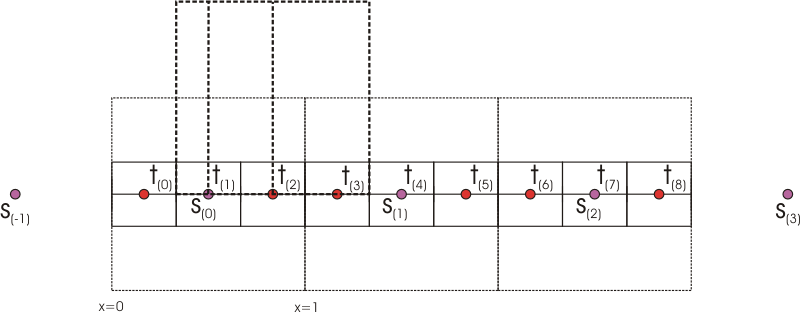
So it picks the source pixel which is the closest to the target pixel (note that there is only one source pixel within a distance of 1/2 of the target pixel). Hence the name of the filter. It is also called a point sampler.

The nearest neighbour resampler

Note that the resampler is not differentiable at the endpoints (|x|=1/2).

Bilinear resampler

f(x) = f1(x)  for |x|<1
     = 0        elsewhere
f1(x) = P * |x| + Q

So, the condition of symmetry is already included above.

These two free parameters are solved by requiring (1) the filter to be continuous and (2) if all the samples are a constant value then the reconstruction should be a flat signal. The latter means that if the source picture has a solid color, then the target picture has the same solid color. This is only possible if the sum of the coefficients of the filter is one.

(1) This means that the value and first derivative are continuous at |x| = 0 and |x| = 1. It results in the following condition:

f1(1) = 0 => P + Q = 0
f1'(0) = constant =>
 f1'(x) = -P for x<=0
 f1'(x) = P for x>=0
 thus for x=0: -P = P => P = 0 (so a continuous derivate can't be possible)

(2) This means that sum_{k=-oo}^oo f(x-k) = 1 for all x:

f1(x) + f1(x+1) = 1 => 2*Q + P = 1

Solving the two conditions gives

> eqn:={P+Q=0, 2*Q+P=1}:
> solve(eqn,{P,Q});
{P=1, Q=-1}

This results in the following bilinear resampler

f(x) = 1 - |x|  for |x|<1
     = 0  elsewhere

The bilinear resampler

Bicubic resampler

Mitchell and Netravali eventually introduced a quite popular family of cubic splines, the BC-splines. A cubic spline filter is in its general form given by

f(x) = f1(x)  for |x|<1
     = f2(x)  for 1<=|x|<2
     = 0        elsewhere
f1(x) = P * |x|^3 + Q * |x|^2 + R * |x| + S
f2(x) = T * |x|^3 + U * |x|^2 + V * |x| + W

So, the condition of symmetry is already included above.

These eight free parameters are reduced to two by requiring (1) the filter to be smooth and (2) if all the samples are a constant value then the reconstruction should be a flat signal. The latter means that if the source picture has a solid color, then the target picture has the same solid color. This is only possible if the sum of the coefficients of the filter is one.

(1) This means that the value and first derivative are continuous at |x| = 0, |x| = 1 and |x| = 2. It results in the following four conditions:

f1(1) = f2(1) => P + Q + R + S = T + U + V + W
f2(2) = 0 => 8*T + 4*U + 2*V + W = 0
f1'(1) = f2'(1) => 3*P + 2*Q + R = 3*T + 2*U + V
f1'(0) = constant =>
 f1'(x) = -3*P*x^2+2*Q*x-R for x<=0
 f1'(x) = 3*P*x^2+2*Q*x+R for x>=0
 thus for x=0: -R = R => R = 0

(2) This means that sum_{k=-oo}^oo f(x-k) = 1 for all x:

f2(x) + f1(x+1) + f1(x+2) + f2(x+3) = 1 =>
(2*U + 9*T + 2*Q + 3*P) * x^2 + (6*U + 27*T + 6*Q + 9*P) x + 27*T + 9*U + 3*V + 2*W + 7*P + 5*Q + R + 2*S = 1

This results in the following two different conditions

(2*U + 9*T + 2*Q + 3*P) = 0
9*T + 5*U + 3*V + 2*W + P + Q + R + 2*S = 1
27*T + 9*U + 3*V + 2*W + 7*P + 5*Q + R + 2*S = 1 (redundant because this holds if the first two conditions are met)

Solving the six equations (in terms of Q and S) using Maple gives:

> eqn:={P+Q+R+S=T+U+V+W, 8*T+4*U+2*V+W=0, 3*P+2*Q+R=3*T+2*U+V, -R=R, 2*U+9*T+2*Q+3*P=0, 9*T+5*U+3*V+2*W+P+Q+R+2*S=1}:
> solve(eqn,{P,R,T,U,V,W});
{Q = Q, S = S, R = 0, P = 1/2 - Q - 3/2 S, T = 5/2 - Q - 11/2 S, V = 18 - 8 Q - 42 S, U = -12 + 5 Q + 27 S, W = -8 + 4 Q + 20 S}

Setting

S = 1 - B/3
Q = -3+2*B+C

gives us the other coefficients as function of B and C:

P = 1/2 - Q - 3/2*S = 2 - 3/2*B - C
T = 5/2 - Q - 11/2*S = - 1/6*B - C
V = 18 - 8*q - 42*s = - 2*B - 8*C
U = -12 + 5*q + 27*s = B + 5*C
W = -8 + 4*q + 20*s = 4/3*B + 4*C

This results in the following family of cubic filters

f(x) = [ (12-9*B-6*C)*|x|^3 + (-18+12*B+6*C)*|x|^2 + (6-2*B) ] / 6  for |x|<1
     = [ (-B-6*C)*|x|^3 + (6*B+30*C)*|x|^2 + (-12*B-48*C)*|x| + (8*B+24*C) ] / 6  for 1<=|x|<2
     = 0  elsewhere

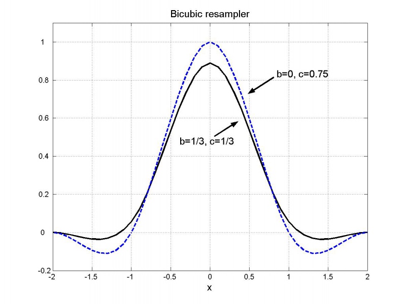
Some of the values for B and C correspond to well known filters (source: 1 2). For example:

B=1, C=0: cubic B-sline;
B=0, C=C: cardinal splines (C=1/2 the Catmull-Rom spline; C=0 the family of Duff's tensioned B-splines)

The bicubic resampler

Windowed sinc resamplers

Windows are used to approximate an "ideal" impulse response of infinite duration, such as a sinc function, to an impuls response of finite duration. Recall that sinc(x) is maximal and equal to one for x=0. It has such a shape that the source pixels closest to the target pixel (that is the center of the resampler) will contribute the most. This implies that the window should also fulfil this property. All windows mentioned here (source) are symmetric, and thus are the resamplers also symmetric.

Sinc resampler

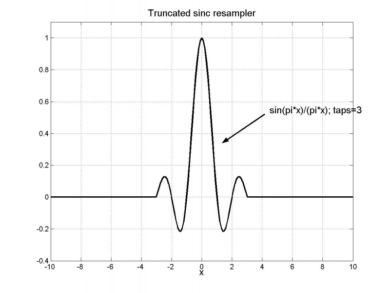
The sinc resampler is just a truncated sinc function. The box window is given by

w(x, taps) = 1  for |x|<taps
           = 0  elsewhere

and the resampler is given by

f(x) = sinc(x) * w(x, taps)

So, the condition of symmetry (and sum_{k=-oo}^oo f(x-k) = 1) is already included above. Note that the resampler is continuous everywhere, but not differentiable at the endpoints (|x|=taps).

The truncated sinc resampler (taps=3)

Lanczos resampler

The Lanczos window is given by

w(x, taps) = sinc(x/taps)  for |x|<taps
           = 0  elsewhere

and the resampler is given by

f(x) = a(taps) * sinc(x) * w(x, taps)

with

sinc(x) = sin(pi*x) / (pi*x)  for x !=0
        = 1  elsewhere

The resampler is differentiable everywhere (also at the points |x|=taps???). a(taps) needs to be chosen such that the following condition is fulfilled:

sum_{k=-oo}^oo f(x-k) = 1  for all x

Note that is a(x, taps) is very close to one for taps>=3.

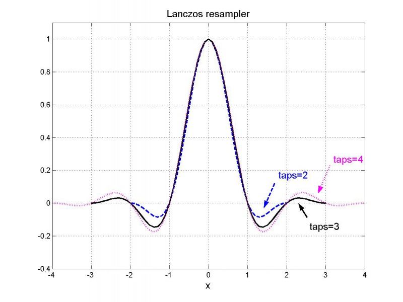
The (unnormalized) lanczos resampler

Blackman resampler

The blackman window is given by

w(x, taps) = (1-a)/2 + 1/2*cos(x/taps) + a/2*cos(2*x/taps)  with a = 0.16  for |x|<taps
           = 0  elsewhere

and the resampler is given by

f(x) = a(taps) * sinc(x) * w(x, taps)

Note that the resampler is continuous everwhere, but not differentiable at the endpoints (|x|=taps). a(taps) needs to be chosen such that the following condition is fulfilled:

sum_{k=-oo}^oo f(x-k) = 1  for all x

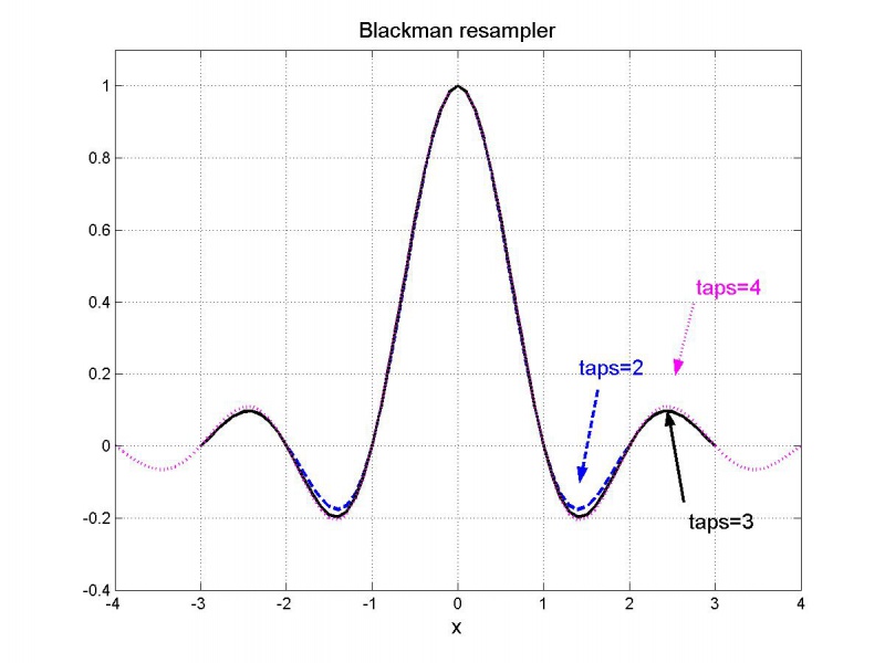
The (unnormalized) blackman resampler

Spline resampler

The Spline16/36/64 resamplers were introduced by Helmut Dersch, the author of Panorama Tools. It fits a cubic spline through the sample points and then derives the filter kernel from the resulting blending polynomials.

Let's consider Spline16 as an example which uses 4 sample points (-1,0,1,2) (the others are derived in a similar way). Consider three (cubic) splines for the interval:

S1(x) = c[3]*x^3 + c[2]*x^2 + c[1]*x + c[0]  for x in [-1,0]
S2(x) = a[3]*x^3 + a[2]*x^2 + a[1]*x + a[0]  for x in [0,1]
S3(x) = b[3]*x^3 + b[2]*x^2 + b[1]*x + b[0]  for x in [1,2]

Let's define (under the condition that the polynomials will be continuous everywhere):

y0 = S1(-1)
y1 = S1(0) = S2(0)
y2 = S2(1) = S3(1)
y3 = S3(2)

Under the condition that the polynomials have continuous first and second derivatives and that the endpoints have a zero second derivative we will get the following additional conditions

S1'(0) = S2'(0)
S2'(1) = S3'(1)
S1''(0) = S2''(0)
S2''(1) = S3''(1)
S1''(-1) = 0
S3''(2) = 0

The coefficients, (a[j])_j, are fixed by these boundary conditions. This results in the following set equations:

-c3 + c2 - c1 + c0 = y0
c0 = y1
a0 = y1
a3 + a2 + a1 + a0 = y2
b3 + b2 + b1 + b0 = y2
8*b3 + 4*b2 + 2*b1 + b0 = y3
c1 - a1 = 0
3*a3 + 2*a2 + a1 - 3*b3 - 2*b2 - b1 = 0
2*c2 - 2*a2 = 0
6*a3 + 2*a2 - 6*b3 - 2*b2 = 0
-6*c3 + 2*c2 = 0
12*b3 + 2*b2 = 0

Solving this set of equations with Maple results in:

> solution:=solve(eqn,{a0,a1,a2,a3,b0,b1,b2,b3,c0,c1,c2,c3}):
> a0s:=subs(solution, a0); a1s:=subs(solution, a1); a2s:=subs(solution, a2); a3s:=subs(solution, a3);
  
a0s := y1
a1s := - 7/15 y0 - 1/5 y1 + 4/5 y2 - 2/15 y3
a2s := 4/5 y0 - 9/5 y1 + 6/5 y2 - 1/5 y3
a3s := - 1/3 y0 + y1 - y2 + 1/3 y3

We are only interested in the spline for [0,1]. The values of the coefficients of the other two splines are not important (so they are not shown here). So, it turns out that the coefficients (a[j])_j (and thus the spline itself) can be expressed as a linear combination of the control points y[j]. This means that

S2(x) = w0(x) * y0 + w1(x) * y1 + w2(x) * y2 + w3(x) * y3

where

w0(x) = - 1/3 * x^3 + 4/5 * x^2 - 7/15 * x
w1(x) = x^3 - 9/5 * x^2 - 1/5 * x + 1
w2(x) = -x^3 + 6/5 * x^2 + 4/5 * x
w3(x) = 1/3 * x^3 - 1/5 * x^2 - 2/15 * x

Since w0,w1,w2,w3 blend the points y0,y1,y2,y3 together, they are called blending polynomials (or basis functions). As a result of the boundary conditions we have:

y1 = S2(0) = w0(0) * y0 + w1(0) * y1 + w2(0) * y2 + w3(0) * y3 => w0(0)=0, w1(0)=1, w2(0)=0, w3(0)=0
y2 = S2(1) = w0(0) * y0 + w1(0) * y1 + w2(0) * y2 + w3(0) * y3 => w0(0)=0, w1(0)=0, w2(0)=1, w3(0)=0

It's also true that the sum of the blending polynomials is equal to one, that is

w0(x) + w1(x) + w2(x) + w3(x) = 1

(The reason is that, if all the y[i] are equal (to k, say), then it is clear that the solution Si(x)=k (for all i,x) satisfies the initial constraints. (Intuitively, interpolating a set of constant values gives that same value.) Since S2(x) = sum_i (wi(x)*y[i]) = k * sum_i wi(x), it follows that the sum of the weights is 1.)

What happens if you replace y[j] by y[3-j] (for j=0,1)? In that case the polynomial S2 will be mirrored at x=1/2, since (1) S2 is fixed by (y0,y1,y2,y3) and (2) z0=z1. In other words:

S2[y0;y1;y2;y3](x) = S2[y3;y2;y1;y0](1-x)

since the mapping x |-> 1-x results in the same mirroring of S2 at x=1/2. It follows that

w2(x) = w1(1-x), w3(x) = w0(1-x)

The filter kernel is defined as

f(x) = w1(x) = x^3 - 9/5 * x^2 - 1/5 * x + 1  for |x|<1
f(x) = w0(x-1) = - 1/3 * (x-1)^3 + 4/5 * (x-1)^2 - 7/15 * (x-1)  for 1<=|x|<2
f(x) = 0  elsewhere

Note that the weights are just continuous, but not continuous differentiable at the joints. In general for Spline k^2 (k even), we start with k-1 bicubic splines. They are located at (-k/2+1,-k/2+2), ..., (k/2-1,k/2). The bending polynomials are calculated from the polynomial located at [0,1], which is expressed as a linear combination of (y0, ..., y(k-1)). The boundary conditions are:

S[1](-k/2+1) = y0
S[1](-k/2+2) = y1
S[2](-k/2+2) = y1
...
S[k-2](k/2-1) = y(k-2)
S[k-2](k/2-1) = y(k-2)
S[k-1](k/2) = y(k-1)

and also continuity of first and second derivatives, where the second derivatives of the two endpoints are zero. This results in k blending functions. More discussion can be found here.

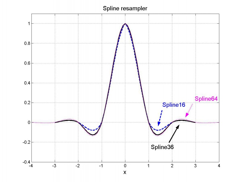
The spline resampler

Gaussian resampler

f(x, q) = a(q) * 2^(-q*x^2)  with q = p*0.1  for |x|<support
        = 0  elsewhere

The support is chosen in such a way that 2^(-q*support^2) = 0, or as an approximation 2^(-q*support^2) = 1.0/512.0 (i.e 0.5 bit). It follows that for example:

p	0.1	5.625	22.5	30	100
support	30.0	4.0	2.0	1.73	0.949

In AviSynth's implementation of GaussResize, it always has support=4.0, regardless of the value of "p". The resampler is differentiable everywhere except at |x|=support. a(q) needs to be chosen such that the following condition is fulfilled:

sum_{k=-oo}^oo f(x-k) = 1  for all x

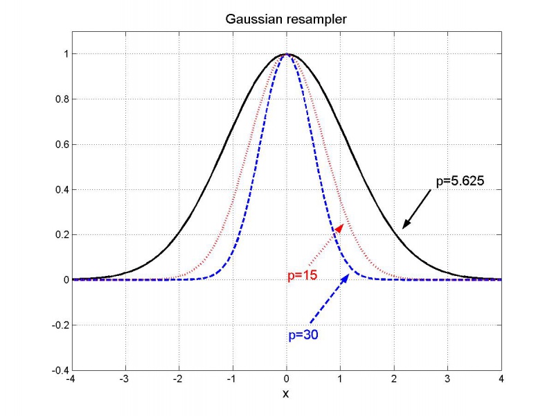
The (unnormalized) gaussian resampler

References

• http://www.ipol.im/pub/art/2011/g_lmii/
• todo: add other relevant articles